The "Trick"

We will now take a closer look at the information of a multi-rotation scan. We know that we have gamma spectra available for a variety of different positions. The positions where the respective measurements were made are also known.

From these individual gamma spectra, we create the sum spectrum. Each channel of the sum spectrum contains the value obtained by adding the contents of that channel for all individual spectra.

We have also learned that the radionuclides contained in the examined container can be identified most quickly based on the characteristic lines in the sum spectrum.

Now we bring all this information together. The fundamental approach is actually quite simple.

• We select one of the characteristic lines identified in the sum spectrum and note its energy.
• Now we look at all individual spectra:
  • We note the position where the examined spectrum was recorded. In the case of a multi-rotation scan, these are the height position and the rotation angle.
  • Next, we check the noted energy to see if a peak is visible in the individual spectrum as well.
    • If yes, we note the number of counts of the peak, i.e., the peak area.
    • If no, we note the value 0 here.
• After examining all individual spectra, we can represent this information in a table – or even better – in a diagram, as can be seen at the top of this page.

Let's consider the procedure in a bit more detail. In the sum spectrum of a multi-rotation scan, we found (among other things) a characteristic line at 59.5 keV. We can assign this to the radionuclide Am-241 using nuclide databases.

The corresponding spatial distribution – this is the term used for the diagram of a characteristic line – is shown below. We want to take a closer look at its components.

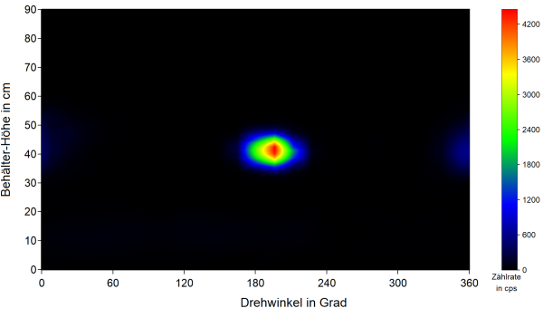
The vertical axis represents the height position, while the horizontal axis represents the rotation angle of the respective measurement position. Since we perform a complete rotation during the multi-rotation scan at each height position, this axis has values between 0 degrees and 360 degrees. The examined container has a height of approximately 86 cm. To ensure we cover all areas of the container, we performed our top measurement slightly above the assumed container height, in this case at a height of 90 cm. Thus, the values of the axis for height positions range between 0 cm (lowest measurement position) and 90 cm (highest measurement position).

In this diagram, we record the number of counts determined for each measurement position (which is defined by specifying the height position and the rotation angle – see Point 2). It has proven advantageous to represent these values with a colored point. Each color corresponds to a specific value or range of values. This type of representation is called “false color representation.” To the right of the diagram, the respective color scale with the assigned value ranges is shown.

How can we use this representation to extract further information?

From the color distribution in the diagram, we can see that at a height of approximately 40 cm and a rotation angle of approximately 190 degrees, the number of counts is significantly increased. From the shape of this circular color distribution, an experienced operator can conclude that there is most likely a point or spherical radioactive source in the container at a height of approximately 40 cm. This source is not in the center of the container but is shifted towards the wall of the container at a rotation angle of approximately 190 degrees.

The described procedure is then repeated for all other characteristic lines of the sum spectrum.

For instance, the diagram at the top right of the page shows the spatial distribution for a characteristic line at 1332.5 keV, which we can assign to Co-60. This diagram exhibits a completely different color distribution compared to the previously discussed diagram for Am-241. It now shows a color strip between a height of approximately 5 cm and 20 cm that is relatively homogeneous across the entire range of rotation angles. An experienced operator would conclude that Co-60 is most likely homogeneously distributed across the entire container cross-section in this layer.

To clarify, here is the fundamental process again as a video (click to start the video): A 200 L container (yellow) contains a spherical source (red). This emits radiation outward. Depending on the position of this source, more or less radiation can be measured on the surface of the container. The “amount” is presented in the video in the so-called false color representation: in the black areas, no radiation can be measured, whereas in the red areas, the most can be measured. In this three-dimensional representation, it is immediately clear where radiation occurs on the surface of the container. The result of such a radiation distribution often needs to be presented in reports. This means that these three-dimensional representations must be depicted in two dimensions. To do this, one “pulls” the distribution off the surface and creates a flat representation from this originally cylindrical representation. Now, with the axes for height and angle positions added – and our spatial distribution is ready.

Admittedly, this was a somewhat difficult topic. Respect if you made it this far and (hopefully) understood it!

Now, let’s briefly summarize what we already know about segmented gamma scanning:

Did you understand the “trick”?

On the next page, we will show you the procedure again using two examples.